Para executar o tutorial abaixo e reproduzir o mapa publicado em Farroñay et al. (2018), é necessário baixar os dados presentes na página https://github.com/ricoperdiz/Tutorials/tree/master/R_map_2018_Farronayetal. Baixe todos os arquivos, com exceção dos arquivos .r e .ipynb (Jupyter Notebook). Baixe o pdf na seção de publicações.

01 Carrega os pacotes

Para manipular os dados e gerar o mapa desta postagem, fiz uso dos pacotes abaixo:

• broom (Robinson, Hayes, e Couch 2022);
• cowplot (Wilke 2020);
• dplyr (Wickham et al. 2021);
• ggsn (Santos Baquero 2019);
• GISTools (Brunsdon e Chen 2014);
• magrittr (Bache e Wickham 2020);
• measurements (Birk 2019);
• purrr (Henry e Wickham 2020);
• readr (Wickham, Hester, e Bryan 2021);
• rgdal (Bivand, Keitt, e Rowlingson 2021);
• sf (Pebesma 2021);
• stringr (Wickham 2019).

Tenha certeza de que todos os pacotes listados abaixo estão instalados.

Atenção especial deve ser dada ao pacote ggmap, que agora requer que seja instalado via GitHub. Veja mais detalhes aqui. Para isso, instale a versão ggmap do GitHub rodando o comando abaixo:

# Rode o comando abaixo para instalar a versao do ggmap do GitHub
# Install ggmap package from GitHub version - this is needed in order to be able to download Google Maps nowadays
# if(!requireNamespace("remotes")) {
#    install.packages("remotes")
#    remotes::install_github("dkahle/ggmap")
#    }

# ----------
## Atencao
# ----------

# ---------------------------------------------------------------
## Todos os dados necessarios para plotar o mapa desta publicacao estao disponiveis em:
# <https://github.com/ricoperdiz/Tutorials/tree/master/R_map_2018_Farronayetal>
## Script author: Ricardo Perdiz <ricardoperdiz@yahoo.com>
## Qualquer duvida ou erro, por favor deixe um alerta em <github.com/ricoperdiz/Tutorials/> ou escreva um email.
# ---------------------------------------------------------------


# lista de pacotes necessarios para rodar este tutorial
package_list <- c("dplyr", "stringr", "readr", "purrr", "magrittr", "broom", "rgdal", "measurements", "GISTools", "ggsn", "cowplot", "sf")

# Rode o comando abaixo para instalar todos os pacotes dentro do vetor package_list
# install.packages(package_list, dependencies = TRUE)

# Carregue os pacotes
libs <- c(package_list, "ggmap")
sapply(libs, library, character.only = TRUE, logical.return = TRUE, quietly = TRUE, warn.conflicts = FALSE)

## Warning: package 'broom' was built under R version 4.1.2

## rgdal: version: 1.5-23, (SVN revision 1121)
## Geospatial Data Abstraction Library extensions to R successfully loaded
## Loaded GDAL runtime: GDAL 3.2.1, released 2020/12/29
## Path to GDAL shared files: /Library/Frameworks/R.framework/Versions/4.1/Resources/library/rgdal/gdal
## GDAL binary built with GEOS: TRUE 
## Loaded PROJ runtime: Rel. 7.2.1, January 1st, 2021, [PJ_VERSION: 721]
## Path to PROJ shared files: /Library/Frameworks/R.framework/Versions/4.1/Resources/library/rgdal/proj
## PROJ CDN enabled: FALSE
## Linking to sp version:1.4-5
## To mute warnings of possible GDAL/OSR exportToProj4() degradation,
## use options("rgdal_show_exportToProj4_warnings"="none") before loading rgdal.
## Overwritten PROJ_LIB was /Library/Frameworks/R.framework/Versions/4.1/Resources/library/rgdal/proj

## Checking rgeos availability: TRUE
## Please note that 'maptools' will be retired by the end of 2023,
## plan transition at your earliest convenience;
## some functionality will be moved to 'sp'.

## Warning: package 'MASS' was built under R version 4.1.2

## 
## Attaching package: 'MASS'

## The following object is masked from 'package:dplyr':
## 
##     select

## rgeos version: 0.5-9, (SVN revision 684)
##  GEOS runtime version: 3.8.1-CAPI-1.13.3 
##  Please note that rgeos will be retired by the end of 2023,
## plan transition to sf functions using GEOS at your earliest convenience.
##  Linking to sp version: 1.4-6 
##  Polygon checking: TRUE

## Linking to GEOS 3.8.1, GDAL 3.2.1, PROJ 7.2.1

## Google's Terms of Service: https://cloud.google.com/maps-platform/terms/.

## Please cite ggmap if you use it! See citation("ggmap") for details.

##        dplyr      stringr        readr        purrr     magrittr        broom 
##         TRUE         TRUE         TRUE         TRUE         TRUE         TRUE 
##        rgdal measurements     GISTools         ggsn      cowplot           sf 
##         TRUE         TRUE         TRUE         TRUE         TRUE         TRUE 
##        ggmap 
##         TRUE

# If any of the messages below points FALSE, it means that you do not have that package installed. So, please install it before proceeding with the tutorial.
# if you do not remember how to install a package, use the command below
# install.packages("PackageName", dependencies = TRUE)

Os pacotes blogdown (Xie, Dervieux, e Presmanes Hill 2021), rmarkdown (Xie, Allaire, e Grolemund 2018), e knitr (Xie 2021) foram utilizados tanto para gerar a estrutura deste sítio web quanto para gerar os arquivos .html que vocês estão lendo neste momento.

02 Lê os dados

Dados para este tutorial se dividem entre dados dos espécimes e dados SIG. Dados de espécimes contêm coordenadas, enquanto dados SIG contêm todos os shapefiles necessários para os mapas.

Dados de espécimes

# Macrolobium longipes
nybg <- read_delim("https://raw.githubusercontent.com/ricoperdiz/Tutorials/master/R_map_2018_Farronayetal/nybg.csv", delim = ",")

## Warning: One or more parsing issues, see `problems()` for details

## Rows: 4 Columns: 33

## ── Column specification ────────────────────────────────────────────────────────
## Delimiter: ","
## chr (20): AdmGUIDValue_tab, DarInstitutionCode, DarDatasetName, DarBasisOfRe...
## dbl  (6): DarCatalogNumber, DarCollector, DarYearCollected, DarDecimalLatitu...
## lgl  (7): DarMinimumElevation, DarMaximumElevation, DarGeorefMethod, DarSubs...

## 
## ℹ Use `spec()` to retrieve the full column specification for this data.
## ℹ Specify the column types or set `show_col_types = FALSE` to quiet this message.

splink <- read_delim("https://raw.githubusercontent.com/ricoperdiz/Tutorials/master/R_map_2018_Farronayetal/splink.csv", delim = ";")

## Rows: 4 Columns: 76

## ── Column specification ────────────────────────────────────────────────────────
## Delimiter: ";"
## chr  (22): institutioncode, kingdom, descrindividuo, aux_nomecompunidgeo_inv...
## dbl   (9): codcolbot, codespecime, numtombo, numcoleta, diacoleta, mescoleta...
## lgl  (43): basisofrecord, phylum, class, ordem, fieldnumber, julianday, time...
## date  (2): datelastmodified, dataultalter

## 
## ℹ Use `spec()` to retrieve the full column specification for this data.
## ℹ Specify the column types or set `show_col_types = FALSE` to quiet this message.

inpa <- read_delim("https://raw.githubusercontent.com/ricoperdiz/Tutorials/master/R_map_2018_Farronayetal/inpa.csv", delim = ",")

## Rows: 2 Columns: 5

## ── Column specification ────────────────────────────────────────────────────────
## Delimiter: ","
## chr (4): COORD_, HERBARIA, COLETOR, ESPECIE
## dbl (1): NUMERO_COL

## 
## ℹ Use `spec()` to retrieve the full column specification for this data.
## ℹ Specify the column types or set `show_col_types = FALSE` to quiet this message.

# Macrolobium aracaense
araca <- read_delim("https://raw.githubusercontent.com/ricoperdiz/Tutorials/master/R_map_2018_Farronayetal/Maracaense.csv", delim = "\t")

## Rows: 2 Columns: 17

## ── Column specification ────────────────────────────────────────────────────────
## Delimiter: "\t"
## chr (10): COLETOR, ADDCOLL, COUNTRY, MINORAREA, MAJORAREA, GAZETTER, COORDEN...
## dbl  (6): NUMERO, COLDD, COLM, COLY, LATITUDE, LONGITUDE
## lgl  (1): SP1

## 
## ℹ Use `spec()` to retrieve the full column specification for this data.
## ℹ Specify the column types or set `show_col_types = FALSE` to quiet this message.

Dados SIG

# South and Central America shape
area_mapa <- rgdal::readOGR(dsn = "SAm_CAm_shape.shp")

## OGR data source with driver: ESRI Shapefile 
## Source: "/Users/ricoperdiz/Documents/PROFISSIONAL/Sites/ricardoperdiz/content/blog/2020_03_29_R-map-Farronayetal-2018/SAm_CAm_shape.shp", layer: "SAm_CAm_shape"
## with 37 features
## It has 65 fields

# Brazilian states shapefile
estados <- st_read("BRASIL.shp")

## Reading layer `BRASIL' from data source 
##   `/Users/ricoperdiz/Documents/PROFISSIONAL/Sites/ricardoperdiz/content/blog/2020_03_29_R-map-Farronayetal-2018/BRASIL.shp' 
##   using driver `ESRI Shapefile'
## Simple feature collection with 27 features and 3 fields
## Geometry type: MULTIPOLYGON
## Dimension:     XY
## Bounding box:  xmin: -73.83943 ymin: -33.77086 xmax: -34.8581 ymax: 5.38289
## CRS:           NA

# Filtra apenas o estado do Amazonas dentro do objeto `estados`
br_amazonas <- estados %>% filter(ESTADO == "Amazonas")
br_amazonas

## Simple feature collection with 1 feature and 3 fields
## Geometry type: MULTIPOLYGON
## Dimension:     XY
## Bounding box:  xmin: -73.68224 ymin: -9.847688 xmax: -55.99345 ymax: 2.198446
## CRS:           NA
##   UF   ESTADO REGIAO                       geometry
## 1 AM Amazonas     NO MULTIPOLYGON (((-63.47887 2...

br_amazonas_tidy <- st_geometry(br_amazonas)
br_amazonas_tidy

## Geometry set for 1 feature 
## Geometry type: MULTIPOLYGON
## Dimension:     XY
## Bounding box:  xmin: -73.68224 ymin: -9.847688 xmax: -55.99345 ymax: 2.198446
## CRS:           NA

## MULTIPOLYGON (((-63.47887 2.198446, -63.43955 2...

area_mapa_tidy <- tidy(area_mapa)

## Regions defined for each Polygons

area_mapa_tidy

## # A tibble: 61,879 × 7
##     long   lat order hole  piece group id   
##    <dbl> <dbl> <int> <lgl> <fct> <fct> <chr>
##  1 -70.0  12.6     1 FALSE 1     0.1   0    
##  2 -69.9  12.5     2 FALSE 1     0.1   0    
##  3 -69.9  12.5     3 FALSE 1     0.1   0    
##  4 -69.9  12.5     4 FALSE 1     0.1   0    
##  5 -69.9  12.5     5 FALSE 1     0.1   0    
##  6 -69.9  12.4     6 FALSE 1     0.1   0    
##  7 -69.9  12.4     7 FALSE 1     0.1   0    
##  8 -69.9  12.4     8 FALSE 1     0.1   0    
##  9 -69.9  12.4     9 FALSE 1     0.1   0    
## 10 -69.9  12.4    10 FALSE 1     0.1   0    
## # … with 61,869 more rows

03 Limpa os dados

Primeiro, limparemos os dados da espécie Macrolobium longipes R.S. Cowan.

# Macrolobium longipes
# first data from inpa
inpa_modif <- inpa %>%
  mutate(
    lat = str_split(COORD_, "N") %>%
      sapply("[[", 1) %>%
      gsub("°", " ", .) %>%
      gsub("’", " ", .) %>%
      paste0(., " 0") %>%
      gsub("  |   ", " ", .) %>%
      str_trim("both") %>%
      measurements::conv_unit(., from = "deg_min_sec", to = "dec_deg"),
    long = str_split(COORD_, "N") %>%
      sapply("[[", 2) %>%
      gsub("°", " ", .) %>%
      gsub("’", " ", .) %>%
      gsub("W", "0", .) %>%
      str_trim("both") %>%
      gsub("  ", " ", .) %>%
      measurements::conv_unit(., from = "deg_min_sec", to = "dec_deg")
  ) %>%
  dplyr::select(-COORD_)
inpa_modif

## # A tibble: 2 × 6
##   HERBARIA COLETOR   NUMERO_COL ESPECIE              lat               long     
##   <chr>    <chr>          <dbl> <chr>                <chr>             <chr>    
## 1 INPA     Huber           5849 Macrolobium longipes 1.58333333333333  66.55    
## 2 INPA     Rodrigues      10875 Macrolobium longipes 0.333333333333333 67.31666…

inpa_modif %>% glimpse()

## Rows: 2
## Columns: 6
## $ HERBARIA   <chr> "INPA", "INPA"
## $ COLETOR    <chr> "Huber", "Rodrigues"
## $ NUMERO_COL <dbl> 5849, 10875
## $ ESPECIE    <chr> "Macrolobium longipes", "Macrolobium longipes"
## $ lat        <chr> "1.58333333333333", "0.333333333333333"
## $ long       <chr> "66.55", "67.3166666666667"

names(inpa_modif) <- tolower(names(inpa_modif)) # turn all column names as lower case
names(inpa_modif)

## [1] "herbaria"   "coletor"    "numero_col" "especie"    "lat"       
## [6] "long"

# then we get speciesLink data and select only columns we want to keep
longipes <- splink %>%
  dplyr::select(
    herbaria = institutioncode,
    coletor, numero_col = numcoleta,
    especie = taxoncompleto,
    pais, estado = estado_prov,
    local = descrlocal
  ) %>%
  # then join them with data from INPA
  full_join(inpa_modif, .) %>%
  dplyr::select(-estado) %>%
  # turn lat and long columns as numeric
  mutate_at(
    .vars = c("lat", "long"),
    .funs = as.numeric
  )

## Joining, by = c("herbaria", "coletor", "numero_col", "especie")

longipes

## # A tibble: 6 × 8
##   herbaria coletor     numero_col especie         lat  long pais   local        
##   <chr>    <chr>            <dbl> <chr>         <dbl> <dbl> <chr>  <chr>        
## 1 INPA     Huber             5849 Macrolobium…  1.58   66.6 <NA>    <NA>        
## 2 INPA     Rodrigues        10875 Macrolobium…  0.333  67.3 <NA>    <NA>        
## 3 JBRJ     Maguire, B.      37590 Macrolobium… NA      NA   Venez… "Rio Siapa, …
## 4 JBRJ     Maguire, B.      37572 Macrolobium… NA      NA   Venez… "Rio Siapa, …
## 5 JBRJ     Maguire, B.      37643 Macrolobium… NA      NA   Venez… "Rio Siapa, …
## 6 JBRJ     Maguire, B.      37590 Macrolobium… NA      NA   Venez… "Rio Siapa, …

longipes %>% glimpse()

## Rows: 6
## Columns: 8
## $ herbaria   <chr> "INPA", "INPA", "JBRJ", "JBRJ", "JBRJ", "JBRJ"
## $ coletor    <chr> "Huber", "Rodrigues", "Maguire, B.", "Maguire, B.", "Maguir…
## $ numero_col <dbl> 5849, 10875, 37590, 37572, 37643, 37590
## $ especie    <chr> "Macrolobium longipes", "Macrolobium longipes", "Macrolobiu…
## $ lat        <dbl> 1.5833333, 0.3333333, NA, NA, NA, NA
## $ long       <dbl> 66.55000, 67.31667, NA, NA, NA, NA
## $ pais       <chr> NA, NA, "Venezuela", "Venezuela", "Venezuela", "Venezuela"
## $ local      <chr> NA, NA, "Rio Siapa, Casiquiare, Territorio Amazonas. ", "Ri…

# at last, we get nybg data and select and rename columns that we want to keep
nybg_modif <- nybg %>%
  dplyr::select(
    herbaria = DarInstitutionCode,
    coletor = DarCollectorNumber,
    numero_col = DarCollector,
    local = DarLocality,
    lat = DarDecimalLatitude,
    long = DarDecimalLongitude,
    pais = DarCountry
  )
nybg_modif

## # A tibble: 4 × 7
##   herbaria coletor         numero_col local                     lat  long pais  
##   <chr>    <chr>                <dbl> <chr>                   <dbl> <dbl> <chr> 
## 1 NY       H. C. de Lima         3279 Alto Rio Negro, Rio U… -0.130 -67.1 Brazil
## 2 NY       B. Maguire           37590 On right bank of Río … NA      NA   Venez…
## 3 NY       B. Maguire           37590 On right bank of Río … NA      NA   Venez…
## 4 NY       W. A. Rodrigues      10875 Alto Rio Negro. Igara…  0.333 -67.3 Brazil

Sempre é bom olhar nossos dados, checar o tipo de variável para cada coluna, quantas observações e quantas variáveis temos em nossos dados. Podemos fazer isso utilizando a função str() do pacote base do R, ou a função glimpse do pacote dplyr. Aqui usarei a função glimpse no conjunto de dados longipes.

glimpse(longipes)

## Rows: 6
## Columns: 8
## $ herbaria   <chr> "INPA", "INPA", "JBRJ", "JBRJ", "JBRJ", "JBRJ"
## $ coletor    <chr> "Huber", "Rodrigues", "Maguire, B.", "Maguire, B.", "Maguir…
## $ numero_col <dbl> 5849, 10875, 37590, 37572, 37643, 37590
## $ especie    <chr> "Macrolobium longipes", "Macrolobium longipes", "Macrolobiu…
## $ lat        <dbl> 1.5833333, 0.3333333, NA, NA, NA, NA
## $ long       <dbl> 66.55000, 67.31667, NA, NA, NA, NA
## $ pais       <chr> NA, NA, "Venezuela", "Venezuela", "Venezuela", "Venezuela"
## $ local      <chr> NA, NA, "Rio Siapa, Casiquiare, Territorio Amazonas. ", "Ri…

glimpse(nybg_modif)

## Rows: 4
## Columns: 7
## $ herbaria   <chr> "NY", "NY", "NY", "NY"
## $ coletor    <chr> "H. C. de Lima", "B. Maguire", "B. Maguire", "W. A. Rodrigu…
## $ numero_col <dbl> 3279, 37590, 37590, 10875
## $ local      <chr> "Alto Rio Negro, Rio Uaupés, Igarapé Tibuarí, acima do Seri…
## $ lat        <dbl> -0.130278, NA, NA, 0.333333
## $ long       <dbl> -67.0892, NA, NA, -67.3167
## $ pais       <chr> "Brazil", "Venezuela", "Venezuela", "Brazil"

longipes <-
  longipes %>%
  full_join(., nybg_modif)

## Joining, by = c("herbaria", "coletor", "numero_col", "lat", "long", "pais", "local")

longipes # now with data from INPA and NY herbaria

## # A tibble: 10 × 8
##    herbaria coletor         numero_col especie      lat  long pais   local      
##    <chr>    <chr>                <dbl> <chr>      <dbl> <dbl> <chr>  <chr>      
##  1 INPA     Huber                 5849 Macrolob…  1.58   66.6 <NA>    <NA>      
##  2 INPA     Rodrigues            10875 Macrolob…  0.333  67.3 <NA>    <NA>      
##  3 JBRJ     Maguire, B.          37590 Macrolob… NA      NA   Venez… "Rio Siapa…
##  4 JBRJ     Maguire, B.          37572 Macrolob… NA      NA   Venez… "Rio Siapa…
##  5 JBRJ     Maguire, B.          37643 Macrolob… NA      NA   Venez… "Rio Siapa…
##  6 JBRJ     Maguire, B.          37590 Macrolob… NA      NA   Venez… "Rio Siapa…
##  7 NY       H. C. de Lima         3279 <NA>      -0.130 -67.1 Brazil "Alto Rio …
##  8 NY       B. Maguire           37590 <NA>      NA      NA   Venez… "On right …
##  9 NY       B. Maguire           37590 <NA>      NA      NA   Venez… "On right …
## 10 NY       W. A. Rodrigues      10875 <NA>       0.333 -67.3 Brazil "Alto Rio …

longipes <-
  longipes %>%
  filter(!is.na(lat), coletor != "Rodrigues") %>%
  # add species name in a separate column
  mutate(
    especie = "M. longipes"
  )
glimpse(longipes)

## Rows: 3
## Columns: 8
## $ herbaria   <chr> "INPA", "NY", "NY"
## $ coletor    <chr> "Huber", "H. C. de Lima", "W. A. Rodrigues"
## $ numero_col <dbl> 5849, 3279, 10875
## $ especie    <chr> "M. longipes", "M. longipes", "M. longipes"
## $ lat        <dbl> 1.583333, -0.130278, 0.333333
## $ long       <dbl> 66.5500, -67.0892, -67.3167
## $ pais       <chr> NA, "Brazil", "Brazil"
## $ local      <chr> NA, "Alto Rio Negro, Rio Uaupés, Igarapé Tibuarí, acima do …

Agora limparemos os dados referentes à espécie nova descrita em Farroñay et al. (2018), chamada Macrolobium aracaense Farroñay.

# Macrolobium aracaense
## Clean data

# turn column names to lower case
names(araca) <- tolower(names(araca))

araca_md <- araca %>%
  mutate(
    # clean coordinate columns to extract and convert degrees min sec to decimal degrees
    lat = str_split(coordenadas, "N") %>%
      sapply("[[", 1) %>%
      gsub("°", " ", .) %>%
      gsub("\'|\'\'|\"", " ", .) %>%
      gsub("  |   ", " ", .) %>%
      str_trim("both") %>%
      measurements::conv_unit(., from = "deg_min_sec", to = "dec_deg"),
    # do the same done for long data
    long = str_split(coordenadas, "N") %>%
      sapply("[[", 2) %>%
      gsub("W", "", .) %>%
      gsub("°", " ", .) %>%
      gsub("\'|\'\'|\"", " ", .) %>%
      gsub("  |   ", " ", .) %>%
      str_trim("both") %>%
      measurements::conv_unit(., from = "deg_min_sec", to = "dec_deg"),
    especie = "M. aracaense"
  ) %>%
  dplyr::select(coletor,
    numero_col = numero,
    pais = country,
    lat, long, estado = majorarea, herbaria, especie
  ) %>%
  # turn lat and long columns as numeric
  mutate_at(
    .vars = c("lat", "long"),
    .funs = as.numeric
  )
glimpse(araca_md)

## Rows: 2
## Columns: 8
## $ coletor    <chr> "Vicentini, A.", "Farroñay, F."
## $ numero_col <dbl> 1886, 178
## $ pais       <chr> "Brasil", "Brasil"
## $ lat        <dbl> 0.9483333, 0.8633333
## $ long       <dbl> 63.39167, 63.33167
## $ estado     <chr> "Amazonas", "Amazonas"
## $ herbaria   <chr> "INPA", "INPA"
## $ especie    <chr> "M. aracaense", "M. aracaense"

# join data for Macrolobium longipes and M. aracaense
dados <-
  full_join(longipes, araca_md) %>%
  dplyr::select(herbaria, coletor, numero_col, especie, lat, long)

## Joining, by = c("herbaria", "coletor", "numero_col", "especie", "lat", "long", "pais")

glimpse(dados)

## Rows: 5
## Columns: 6
## $ herbaria   <chr> "INPA", "NY", "NY", "INPA", "INPA"
## $ coletor    <chr> "Huber", "H. C. de Lima", "W. A. Rodrigues", "Vicentini, A.…
## $ numero_col <dbl> 5849, 3279, 10875, 1886, 178
## $ especie    <chr> "M. longipes", "M. longipes", "M. longipes", "M. aracaense"…
## $ lat        <dbl> 1.5833333, -0.1302780, 0.3333330, 0.9483333, 0.8633333
## $ long       <dbl> 66.55000, -67.08920, -67.31670, 63.39167, 63.33167

dados$long <- ifelse(dados$long > 0, dados$long * -1, dados$long)
longipes <- dados %>%
  filter(especie == "M. longipes")
aracaense <- dados %>%
  filter(especie == "M. aracaense")

Agora temos dois objetos contendo os dados necessários para cada espécie, Macrolobium longipes e M. aracaense.

longipes

## # A tibble: 3 × 6
##   herbaria coletor         numero_col especie        lat  long
##   <chr>    <chr>                <dbl> <chr>        <dbl> <dbl>
## 1 INPA     Huber                 5849 M. longipes  1.58  -66.6
## 2 NY       H. C. de Lima         3279 M. longipes -0.130 -67.1
## 3 NY       W. A. Rodrigues      10875 M. longipes  0.333 -67.3

aracaense

## # A tibble: 2 × 6
##   herbaria coletor       numero_col especie        lat  long
##   <chr>    <chr>              <dbl> <chr>        <dbl> <dbl>
## 1 INPA     Vicentini, A.       1886 M. aracaense 0.948 -63.4
## 2 INPA     Farroñay, F.         178 M. aracaense 0.863 -63.3

04 Cria variáveis para o mapa

# longitude range - main map
x1 <- st_bbox(br_amazonas)[c(1, 3)]
x1

##      xmin      xmax 
## -73.68224 -55.99345

y1 <- st_bbox(br_amazonas)[c(2, 4)]
y1

##      ymin      ymax 
## -9.847688  2.198446

# longitude and latitude range - for ggmap
lat_long <- dados
y_geral <- range(lat_long$lat) + c(-0.01, 0.01)
y_geral

## [1] -0.140278  1.593333

x_geral <- range(lat_long$long) + c(-0.01, 0.01)
x_geral

## [1] -67.32670 -63.32167

05 Baixa o mapa via pacote R ggmap

Recentemente, houve uma mudança na maneira de baixar mapas Google através do pacote ggmap. Agora é necessária a obtenção de uma chave Google e utiizá-la ao rodar os comandos abaixo com a função mostrada abaixo. Após ese passo, o usuário terá a permissão de baixar os mapas Google usando a função ggmap::get_map.

Para mais informações, visite este sítio web.

# Place your google KEY here - without it, you WILL NOT be able to download a google map
# register_google(key = 'PlaceYourKeyRightHERE!')

# local_mp <- c(lon = sum(x_geral)/2, lat = sum(y_geral)/2)
# local_mp
# mapa <- get_map(location = local_mp,
#        source = "google",
#        maptype = "terrain", crop = FALSE,
#        zoom = 7,
#        color = 'bw',
#        language = 'en-EN')

Para checar se funcionou, tente plotar o objeto mapa:

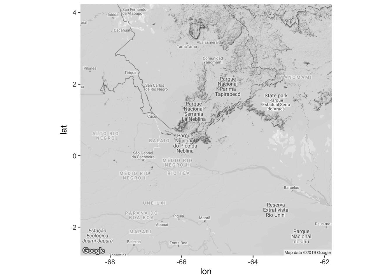
mapa

Se você não obteve sucesso em baixar o mapa, utilize o arquivo .RDS abaixo para poder prosseguir com o tutorial. Ele contem exatamente o mesmo mapa baixado do Google utilizado na publicação, e se encontra disponível na pasta https://github.com/ricoperdiz/Tutorials/tree/master/R_map_2018_Farronayetal.

mapa <- readRDS("Farronayetal2017_ggmap.RDS")

ggmap(mapa, extent = "panel")

06 Plotam-se os mapas

# Main map - species distribution
x_escala <- -65.1

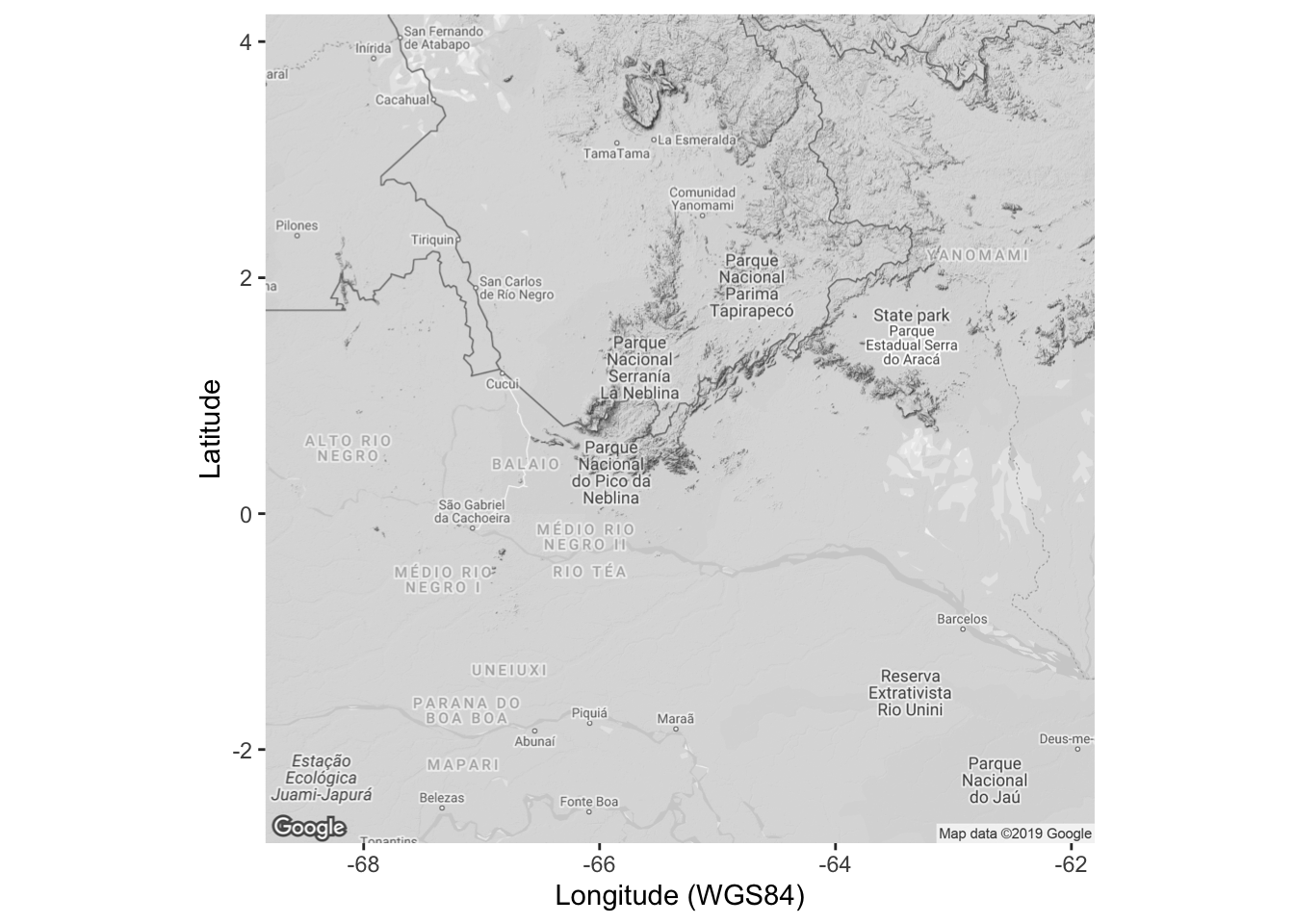
araca_map1 <-
  ggmap(mapa, extent = "panel") +
  xlab("Longitude (WGS84)") +
  ylab("Latitude")
# plot the map with X and Y Label on it
# take a first look to see if everything is all right
araca_map1

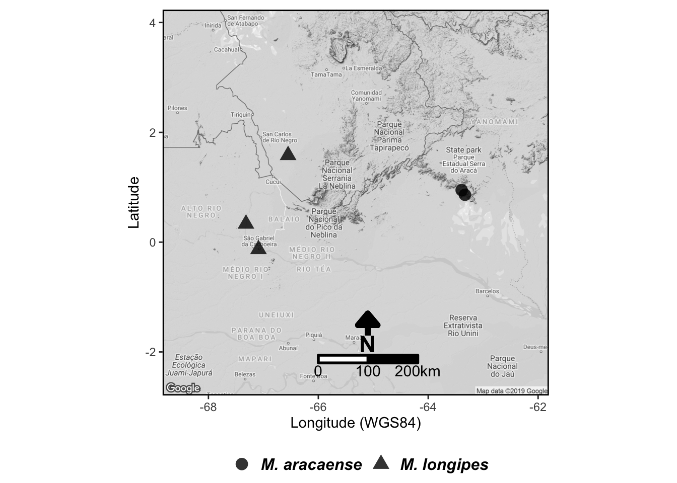
# Main map
araca_map <-
  araca_map1 +
  geom_point(aes(x = long, y = lat, shape = especie), data = dados, alpha = .8, color = "black", size = 4) +
  # add scale bar on topleft
  scalebar(
    x.min = attr(mapa, "bb")[[2]],
    y.min = attr(mapa, "bb")[[1]],
    x.max = attr(mapa, "bb")[[4]],
    y.max = attr(mapa, "bb")[[3]],
    dist = 100, anchor = c(x = -66, y = -2.2),
    model = "WGS84",
    location = "topleft",
    st.size = 4,
    st.dist = 0.02,
    transform = TRUE,
    dist_unit = "km"
  ) +
  # add North arrow
  geom_segment(
    arrow = arrow(length = unit(4, "mm"), type = "closed", angle = 40),
    aes(x = x_escala, xend = x_escala, y = -1.7, yend = -1.3), colour = "black", size = 2
  ) +
  annotate(
    x = x_escala, y = -1.85, label = "N", color = "black", geom = "text", size = 6,
    fontface = "bold"
  ) +
  # change ggplot2 theme to Black and White
  theme_bw() +
  # change few details:
  # color contour of panel border, legend position, plot margin etc
  theme(
    panel.border = element_rect(colour = "black", fill = NA, size = 1),
    legend.title = element_blank(), legend.text = element_text(size = 12, face = "bold.italic"),
    legend.position = "bottom",
    plot.margin = unit(x = c(0.1, 0.1, 0, 0.1), units = "in")
  )

araca_map

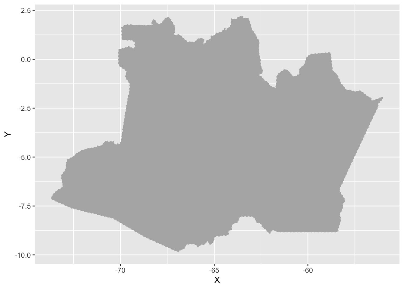
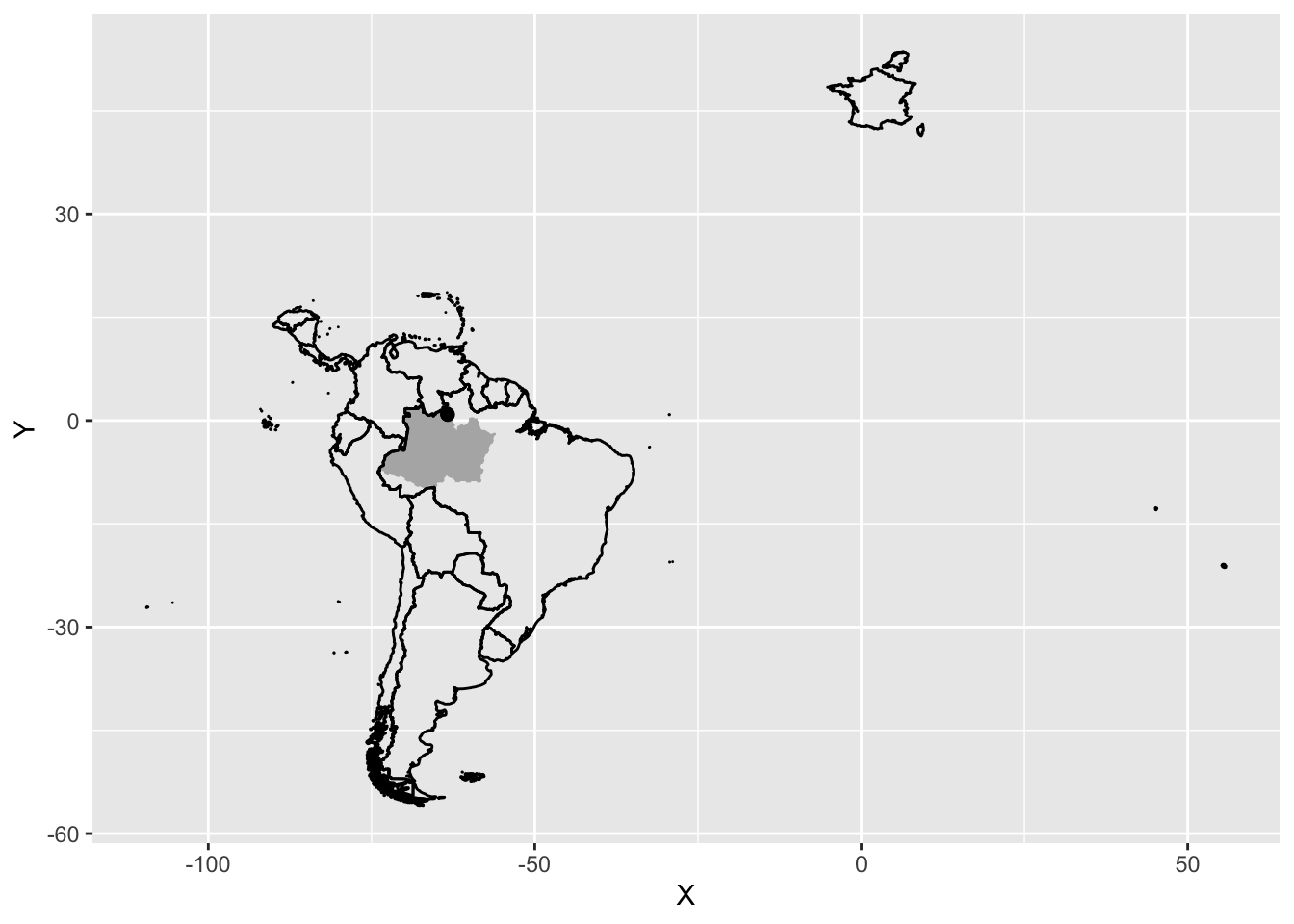
# plot the overview map
overviewmap1 <-
  ggplot() +
  geom_polygon(
    data = as_tibble(st_coordinates(br_amazonas_tidy)),
    aes(x = X, y = Y, group = L1),
    color = "gray70", fill = "gray70", linetype = 3
  )
overviewmap1

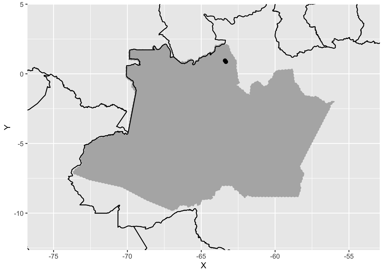
overviewmap2 <- overviewmap1 +
  geom_polygon(
    data = area_mapa_tidy,
    aes(x = long, y = lat, group = group),
    color = "black", fill = NA
  ) +
  geom_point(
    data = subset(dados, especie %in% "M. aracaense"),
    aes(x = long, y = lat), size = 2,
    pch = 19, col = "black"
  )
overviewmap2

overviewmap3 <- overviewmap2 +
  coord_equal() +
  coord_cartesian(
    xlim = x1 - c(2, -2), ylim = y1 - c(2, -2)
  )

## Coordinate system already present. Adding new coordinate system, which will replace the existing one.

overviewmap3

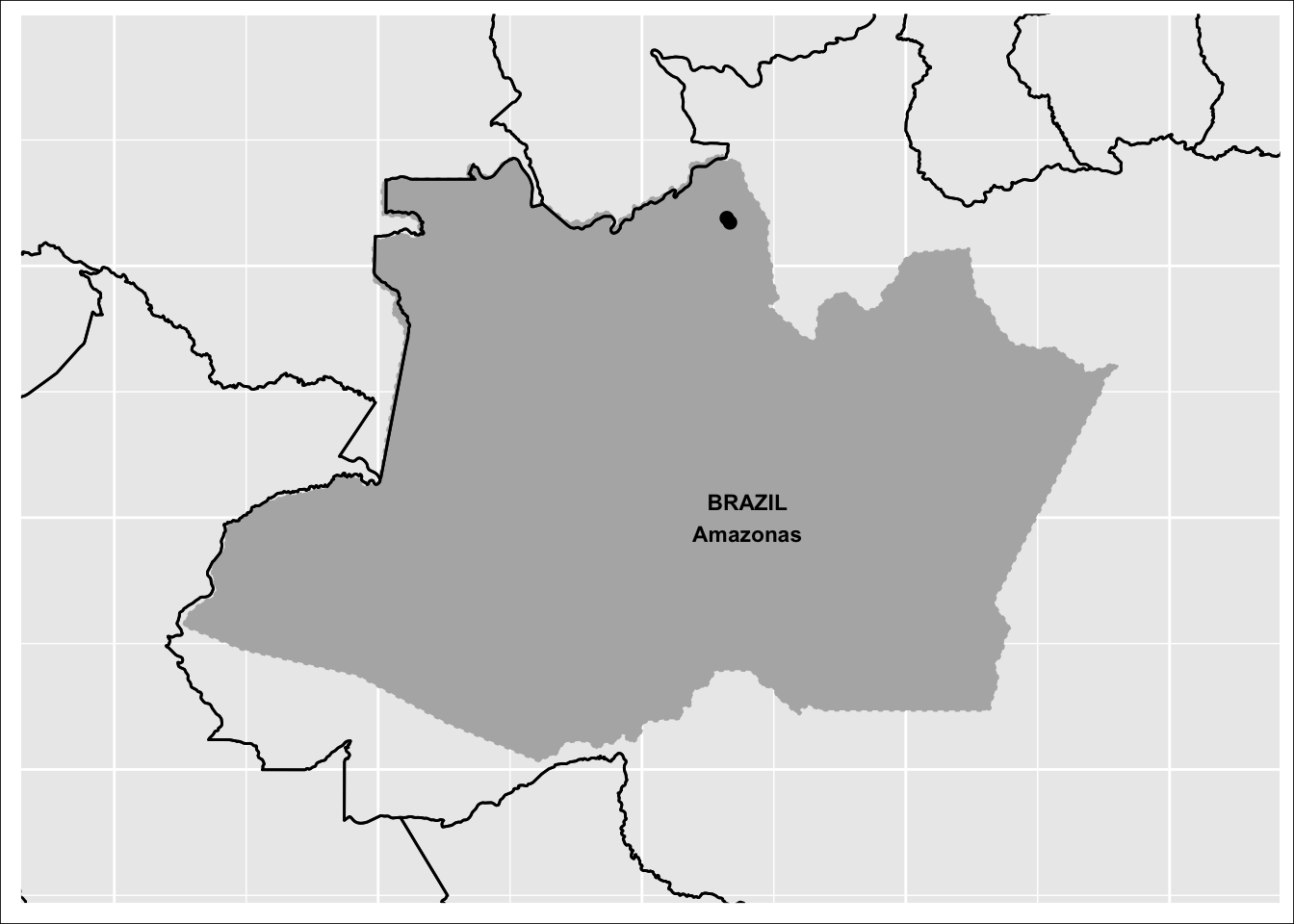
overviewmap <- overviewmap3 +
  theme(
    plot.background =
      element_rect(
        fill = "white", linetype = 1,
        size = 0.3, colour = "black"
      ),
    axis.line = element_blank(),
    axis.text.x = element_blank(),
    axis.text.y = element_blank(),
    axis.ticks = element_blank(),
    axis.title.x = element_blank(),
    axis.title.y = element_blank(),
    legend.position = "none"
  ) +
  annotate(
    x = -63, y = -5, label = "BRAZIL\nAmazonas",
    color = "black", geom = "text",
    size = 3, fontface = "bold"
  )
overviewmap

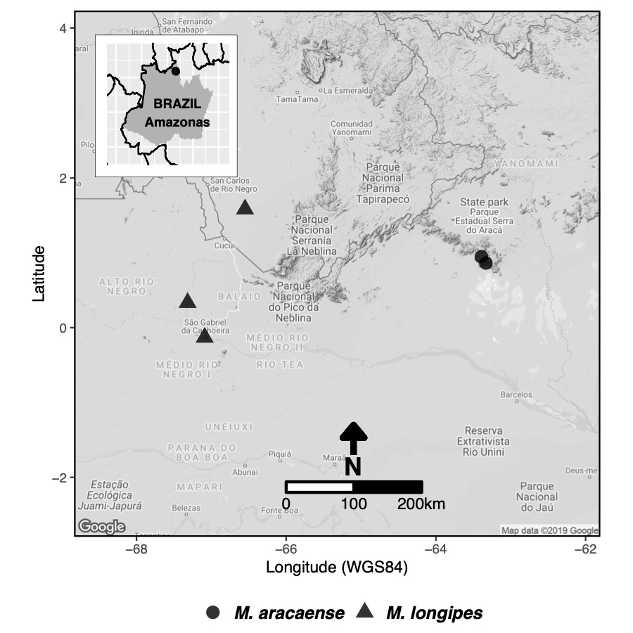
07 Combinam-se os mapas com o pacote R cowplot

final_map <- ggdraw() +
  draw_plot(araca_map, 0, 0, 1, 1) +
  draw_plot(overviewmap, 0.15, 0.72, 0.225, 0.225)
final_map

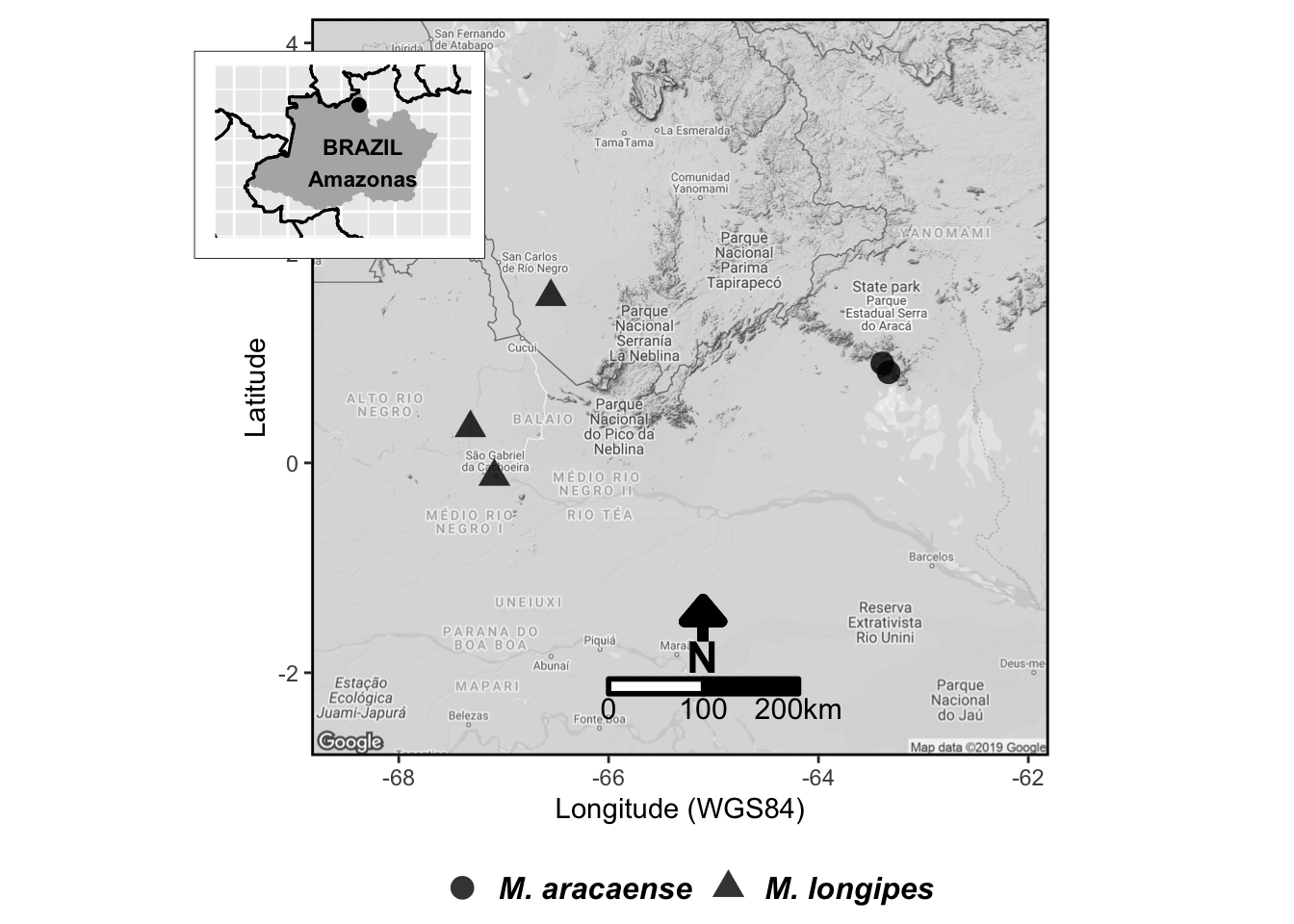
08 Salva o mapa final localmente

cowplot::ggsave2(
  plot = final_map,
  filename = "final_map_Macrolobium_aracaense_ggmap.pdf", dpi = 600, width = 6, height = 6, units = "in"
)

Compare agora a imagem produzida aqui (veja abaixo!) com a publicada em Farroñay et al. (2018).

Referências